Note
Go to the end to download the full example code.
A simple optimization problem: hanging chain#
Again, this example illustrates another simple use of csnlp.Nlp in solving an
optimization problem.
The problem reproduces the example from this CasADi blog post, where a chain of \(N\) point masses (of mass \(m\)) connected by springs is hanging. We are interested in finding the rest position of each of the masses, i.e., \((x_i, y_i), \ i = 1, \ldots, N\). To do so, we minimize the potential energy of the system, which is given by the gravitational potential energy and the elastic energy of the springs
Creating and solving the problem#
Again, the only novel import is csnlp.Nlp. The rest should be familiar.
As last setup step, we define the constant parameters of the problem and create a
matplotlib.figure.Figure with three subplots (which will be populated with
three variants of the problem).
In order to build the optimization problem, we first create an instance of
csnlp.Nlp and define the position variables \(p=(x,y)\). Then, we can
formulate an adequate objective function, i.e., the total energy of the system, and
pass it to the csnlp.Nlp.minimize method.
nlp = Nlp[cs.SX]()
p = nlp.variable("p", (2, N))[0]
x, y = p[0, :], p[1, :]
V = D * (cs.sumsqr(cs.diff(x)) + cs.sumsqr(cs.diff(y))) + g * m * cs.sum2(y)
nlp.minimize(V)
To have the problem well-posed, we need to add some constraints. We fix the first and last points of the chain to be at \((-2, 1)\) and \((2, 1)\), respectively.
nlp.constraint("c1", p[:, 0], "==", [-2, 1])
_ = nlp.constraint("c2", p[:, -1], "==", [2, 1])
We can now solve the problem and plot the chain. We first initialize the solver with
the default options (uses IPOPT) and then call the csnlp.Nlp.solve method.
The solution allows us to compute the numerical value of the optimal positions via
csnlp.Solution.value.
nlp.init_solver()
sol1 = nlp.solve()
******************************************************************************
This program contains Ipopt, a library for large-scale nonlinear optimization.
 Ipopt is released as open source code under the Eclipse Public License (EPL).
         For more information visit https://github.com/coin-or/Ipopt
******************************************************************************

This is Ipopt version 3.14.11, running with linear solver MUMPS 5.4.1.

Number of nonzeros in equality constraint Jacobian...:        4
Number of nonzeros in inequality constraint Jacobian.:        0
Number of nonzeros in Lagrangian Hessian.............:      158

Total number of variables............................:       80
                     variables with only lower bounds:        0
                variables with lower and upper bounds:        0
                     variables with only upper bounds:        0
Total number of equality constraints.................:        4
Total number of inequality constraints...............:        0
        inequality constraints with only lower bounds:        0
   inequality constraints with lower and upper bounds:        0
        inequality constraints with only upper bounds:        0

iter    objective    inf_pr   inf_du lg(mu)  ||d||  lg(rg) alpha_du alpha_pr  ls
   0  0.0000000e+00 2.00e+00 9.81e+00  -1.0 0.00e+00    -  0.00e+00 0.00e+00   0
   1  8.8186499e+02 0.00e+00 1.88e-12  -1.0 2.00e+00    -  1.00e+00 1.00e+00h  1

Number of Iterations....: 1

                                   (scaled)                 (unscaled)
Objective...............:   8.8186498614468883e+02    8.8186498614468883e+02
Dual infeasibility......:   1.8758328224066645e-12    1.8758328224066645e-12
Constraint violation....:   0.0000000000000000e+00    0.0000000000000000e+00
Variable bound violation:   0.0000000000000000e+00    0.0000000000000000e+00
Complementarity.........:   0.0000000000000000e+00    0.0000000000000000e+00
Overall NLP error.......:   7.7613257167867185e-13    1.8758328224066645e-12


Number of objective function evaluations             = 2
Number of objective gradient evaluations             = 2
Number of equality constraint evaluations            = 2
Number of inequality constraint evaluations          = 0
Number of equality constraint Jacobian evaluations   = 2
Number of inequality constraint Jacobian evaluations = 0
Number of Lagrangian Hessian evaluations             = 1
Total seconds in IPOPT                               = 0.003

EXIT: Optimal Solution Found.
solver_ipopt_Nlp0  :   t_proc      (avg)   t_wall      (avg)    n_eval
            nlp_f  |  10.00us (  5.00us)   5.52us (  2.76us)         2
            nlp_g  |  13.00us (  6.50us)   5.93us (  2.97us)         2
       nlp_grad_f  |  31.00us ( 10.33us)  15.06us (  5.02us)         3
       nlp_hess_l  |   7.00us (  7.00us)   3.81us (  3.81us)         1
        nlp_jac_g  |   9.00us (  3.00us)   4.26us (  1.42us)         3
            total  |   7.90ms (  7.90ms)   3.95ms (  3.95ms)         1
Adding ground constraints#
We can further improve the “simulation” of the chain in case it lays on the
hypothetical ground. We can add a new constraint modelling the ground, without the
need to recreate the csnlp.Nlp instance or reinitialize the solver (this is
done manually under the hood). We can also warm-start the new solver’s run with the
previous solution.
nlp.constraint("c3", y, ">=", cs.cos(0.1 * x) - 0.5)
sol2 = nlp.solve(vals0={"p": sol1.vals["p"]})
This is Ipopt version 3.14.11, running with linear solver MUMPS 5.4.1.

Number of nonzeros in equality constraint Jacobian...:        4
Number of nonzeros in inequality constraint Jacobian.:       80
Number of nonzeros in Lagrangian Hessian.............:      158

Total number of variables............................:       80
                     variables with only lower bounds:        0
                variables with lower and upper bounds:        0
                     variables with only upper bounds:        0
Total number of equality constraints.................:        4
Total number of inequality constraints...............:       40
        inequality constraints with only lower bounds:        0
   inequality constraints with lower and upper bounds:        0
        inequality constraints with only upper bounds:       40

iter    objective    inf_pr   inf_du lg(mu)  ||d||  lg(rg) alpha_du alpha_pr  ls
   0  8.8186499e+02 1.66e-01 5.00e-01  -1.0 0.00e+00    -  0.00e+00 0.00e+00   0
   1  8.8660392e+02 0.00e+00 3.75e+00  -1.7 1.68e-01    -  2.09e-01 1.00e+00h  1
   2  8.8668942e+02 0.00e+00 1.47e-02  -1.7 3.26e-02    -  9.92e-01 1.00e+00f  1
   3  8.8607417e+02 0.00e+00 5.01e-08  -2.5 1.13e-02    -  1.00e+00 1.00e+00f  1
   4  8.8600489e+02 0.00e+00 5.75e-02  -3.8 3.45e-03    -  1.00e+00 8.82e-01f  1
   5  8.8599905e+02 0.00e+00 1.92e-08  -3.8 1.04e-03    -  1.00e+00 1.00e+00f  1
   6  8.8599633e+02 0.00e+00 1.43e-02  -5.7 3.32e-04    -  1.00e+00 9.18e-01f  1
   7  8.8599619e+02 0.00e+00 1.23e-10  -5.7 4.94e-05    -  1.00e+00 1.00e+00f  1
   8  8.8599616e+02 0.00e+00 4.03e-13  -8.6 3.57e-06    -  1.00e+00 1.00e+00f  1

Number of Iterations....: 8

                                   (scaled)                 (unscaled)
Objective...............:   3.0851651967586099e+02    8.8599615906914005e+02
Dual infeasibility......:   4.0315217175472610e-13    1.1577703393981887e-12
Constraint violation....:   0.0000000000000000e+00    0.0000000000000000e+00
Variable bound violation:   0.0000000000000000e+00    0.0000000000000000e+00
Complementarity.........:   8.4342836513357344e-09    2.4221532537169310e-08
Overall NLP error.......:   8.4342836513357344e-09    2.4221532537169310e-08


Number of objective function evaluations             = 9
Number of objective gradient evaluations             = 9
Number of equality constraint evaluations            = 9
Number of inequality constraint evaluations          = 9
Number of equality constraint Jacobian evaluations   = 9
Number of inequality constraint Jacobian evaluations = 9
Number of Lagrangian Hessian evaluations             = 8
Total seconds in IPOPT                               = 0.010

EXIT: Optimal Solution Found.
solver_ipopt_Nlp0  :   t_proc      (avg)   t_wall      (avg)    n_eval
            nlp_f  |  50.00us (  5.56us)  23.90us (  2.66us)         9
            nlp_g  |  78.00us (  8.67us)  37.19us (  4.13us)         9
       nlp_grad_f  |  82.00us (  8.20us)  40.03us (  4.00us)        10
       nlp_hess_l  | 106.00us ( 13.25us)  53.21us (  6.65us)         8
        nlp_jac_g  | 107.00us ( 10.70us)  51.48us (  5.15us)        10
            total  |  21.53ms ( 21.53ms)  10.77ms ( 10.77ms)         1
Non-zero rest length#
The problem can be further extended by considering that the springs have a non-zero
rest length. This can be done by modifying the spring energy contributions. We can
then pass the new objective to the csnlp.Nlp.minimize method and solve the
problem again.
This is Ipopt version 3.14.11, running with linear solver MUMPS 5.4.1.

Number of nonzeros in equality constraint Jacobian...:        4
Number of nonzeros in inequality constraint Jacobian.:       80
Number of nonzeros in Lagrangian Hessian.............:      276

Total number of variables............................:       80
                     variables with only lower bounds:        0
                variables with lower and upper bounds:        0
                     variables with only upper bounds:        0
Total number of equality constraints.................:        4
Total number of inequality constraints...............:       40
        inequality constraints with only lower bounds:        0
   inequality constraints with lower and upper bounds:        0
        inequality constraints with only upper bounds:       40

iter    objective    inf_pr   inf_du lg(mu)  ||d||  lg(rg) alpha_du alpha_pr  ls
   0  7.2088397e+02 0.00e+00 1.76e+00  -1.0 0.00e+00    -  0.00e+00 0.00e+00   0
   1  6.2989040e+02 0.00e+00 3.53e+00  -1.0 6.35e-01    -  1.00e+00 7.80e-01f  1
   2  6.3210781e+02 0.00e+00 3.28e-02  -1.0 4.93e-02    -  1.00e+00 1.00e+00f  1
   3  6.2732676e+02 0.00e+00 2.91e-02  -1.7 4.68e-02    -  1.00e+00 1.00e+00f  1
   4  6.2655438e+02 0.00e+00 4.70e-02  -2.5 1.35e-02    -  1.00e+00 9.28e-01f  1
   5  6.2653995e+02 0.00e+00 2.45e-03  -2.5 3.07e-03    -  1.00e+00 1.00e+00f  1
   6  6.2646745e+02 0.00e+00 2.62e-02  -3.8 2.58e-03    -  1.00e+00 9.40e-01f  1
   7  6.2646522e+02 0.00e+00 1.76e-04  -3.8 4.72e-04    -  1.00e+00 1.00e+00f  1
   8  6.2646200e+02 0.00e+00 2.02e-03  -5.7 1.93e-04    -  1.00e+00 9.78e-01f  1
   9  6.2646195e+02 0.00e+00 1.30e-07  -5.7 9.00e-06    -  1.00e+00 1.00e+00f  1
iter    objective    inf_pr   inf_du lg(mu)  ||d||  lg(rg) alpha_du alpha_pr  ls
  10  6.2646191e+02 0.00e+00 1.54e-09  -8.6 2.09e-06    -  1.00e+00 1.00e+00f  1

Number of Iterations....: 10

                                   (scaled)                 (unscaled)
Objective...............:   2.8845353784942159e+02    6.2646191425246241e+02
Dual infeasibility......:   1.5360547463943889e-09    3.3359958210155094e-09
Constraint violation....:   0.0000000000000000e+00    0.0000000000000000e+00
Variable bound violation:   0.0000000000000000e+00    0.0000000000000000e+00
Complementarity.........:   3.9757695974654926e-09    8.6345560232135268e-09
Overall NLP error.......:   3.9757695974654926e-09    8.6345560232135268e-09


Number of objective function evaluations             = 11
Number of objective gradient evaluations             = 11
Number of equality constraint evaluations            = 11
Number of inequality constraint evaluations          = 11
Number of equality constraint Jacobian evaluations   = 11
Number of inequality constraint Jacobian evaluations = 11
Number of Lagrangian Hessian evaluations             = 10
Total seconds in IPOPT                               = 0.011

EXIT: Optimal Solution Found.
solver_ipopt_Nlp0  :   t_proc      (avg)   t_wall      (avg)    n_eval
            nlp_f  |  91.00us (  8.27us)  44.16us (  4.01us)        11
            nlp_g  |  96.00us (  8.73us)  45.34us (  4.12us)        11
       nlp_grad_f  | 134.00us ( 11.17us)  66.12us (  5.51us)        12
       nlp_hess_l  | 426.00us ( 42.60us) 212.69us ( 21.27us)        10
        nlp_jac_g  |  97.00us (  8.08us)  48.46us (  4.04us)        12
            total  |  23.14ms ( 23.14ms)  11.57ms ( 11.57ms)         1
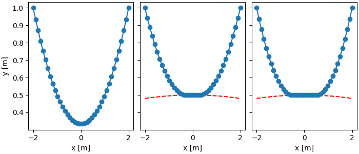
Plotting#
Finally, we can plot the three variants of the chain problem side by side.
def plot_chain(ax: Axes, x: cs.DM, y: cs.DM) -> None:
    ax.plot(x.full().flat, y.full().flat, "o-")


def plot_ground(ax: Axes) -> None:
    xs = np.linspace(-2, 2, 100)
    ax.plot(xs, np.cos(0.1 * xs) - 0.5, "r--")


_, axs = plt.subplots(1, 3, sharey=True, constrained_layout=True, figsize=(7, 3))
plot_chain(axs[0], sol1.value(x), sol1.value(y))
plot_ground(axs[1])
plot_chain(axs[1], sol2.value(x), sol2.value(y))
plot_ground(axs[2])
plot_chain(axs[2], sol3.value(x), sol3.value(y))
axs[0].set_ylabel("y [m]")
for ax in axs:
    ax.set_xlabel("x [m]")
plt.show()
Total running time of the script: (0 minutes 0.440 seconds)