Note
Go to the end to download the full example code.
Simple open-loop MPC controller#
This example demos how an MPC controller can be built via csnlp.wrappers.Mpc
and how it can be solved in an open-loop fashion.
We’ll skip over some of the formalities of the library, as we assume you are already a
bit familiar with it. If this is not the case, for more introductory examples on
csnlp, see the other Introductory examples.
The problem is inspired by the example from this CasADi video, where an optimal control problem for a 2-dimensional task is tackled. The goal is to regulate the state and action towards the origin.In mathematical terms, the state at time \(k\) is indicated by \(x_k\), and evolves according to the continuous-time dynamics
where \(u\) is the control action. We discretize the continuous-time dynamics using a Runge-Kutta 4th order integrator, and we refer to the discrete-time dynamics as \(f_d(x_k,u_k)\). Lastly, we formulate the optimal control problem
Multiple shooting MPC#
In this section we’ll first solve the problem in a multiple shooting formulation (the one proposed above). We start with the usual imports.
import casadi as cs
import matplotlib.pyplot as plt
import numpy as np

from csnlp import Nlp, wrappers
We then define the continuous-time dynamics and discretize them via RK4. The final dynamics are conveniently packed in the function \(F\).
x = cs.MX.sym("x", 2)
u = cs.MX.sym("u")
ode = cs.vertcat((1 - x[1] ** 2) * x[0] - x[1] + u, x[0])
f = cs.Function("f", [x, u], [ode], ["x", "u"], ["ode"])
T = 15
N = 20
intg_options = {"simplify": True, "number_of_finite_elements": 4}
dae = {"x": x, "p": u, "ode": f(x, u)}
intg = cs.integrator("intg", "rk", dae, 0, T / N, intg_options)
res = intg(x0=x, p=u)
x_next = res["xf"]
F = cs.Function("F", [x, u], [x_next], ["x", "u"], ["x_next"])
Then, we can move to building the MPC. Since it is a non-retroactive wrapper, an
fresh csnlp.Nlp instance must be passed to it. Instead of using
csnlp.Nlp.variable, the wrapper exposes two convienient methods to define
states and actions: csnlp.wrappers.Mpc.state and
csnlp.wrappers.Mpc.action. We’ll use those, and also pass some lower- and
upper-bounds to them. After creation of states and actions, we can set the dynamics
via a convenient method csnlp.wrappers.Mpc.set_nonlinear_dynamics that will
automatically add the initial state constraint and the dynamics constraints. Lastly,
an appropriate cost function is defined and the solver is initialized.
mpc = wrappers.Mpc[cs.SX](
    nlp=Nlp[cs.SX](sym_type="SX"), prediction_horizon=N, shooting="multi"
)
u, _ = mpc.action("u", lb=-1, ub=+1)
x, _ = mpc.state("x", 2, lb=-0.2)  # must be created before dynamics
mpc.set_nonlinear_dynamics(F)
mpc.minimize(cs.sumsqr(x) + cs.sumsqr(u))
Before solving, the solver is initialized, and then called with the value of the
initial state x_0, which has been defined as a parameter by
csnlp.wrappers.Mpc.set_nonlinear_dynamics.
opts = {"print_time": False, "ipopt": {"sb": "yes", "print_level": 5}}
mpc.init_solver(opts)
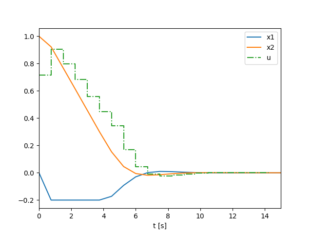
sol = mpc.solve(pars={"x_0": [0, 1]})
t = np.linspace(0, T, N + 1)
plt.plot(t, sol.value(x).T)
plt.step(t[:-1], sol.vals["u"].T.full(), "-.", where="post")
plt.legend(["x1", "x2", "u"])
plt.xlim(t[0], t[-1])
plt.xlabel("t [s]")
plt.show()

This is Ipopt version 3.14.11, running with linear solver MUMPS 5.4.1.

Number of nonzeros in equality constraint Jacobian...:      162
Number of nonzeros in inequality constraint Jacobian.:        0
Number of nonzeros in Lagrangian Hessian.............:      122

Total number of variables............................:       62
                     variables with only lower bounds:       42
                variables with lower and upper bounds:       20
                     variables with only upper bounds:        0
Total number of equality constraints.................:       42
Total number of inequality constraints...............:        0
        inequality constraints with only lower bounds:        0
   inequality constraints with lower and upper bounds:        0
        inequality constraints with only upper bounds:        0

iter    objective    inf_pr   inf_du lg(mu)  ||d||  lg(rg) alpha_du alpha_pr  ls
   0  0.0000000e+00 1.00e+00 1.50e+00  -1.0 0.00e+00    -  0.00e+00 0.00e+00   0
   1  7.3103789e-01 6.32e-01 1.17e+00  -1.0 1.28e+00    -  1.80e-01 3.68e-01h  1
   2  1.7156336e+00 4.52e-01 1.31e+00  -1.0 6.91e-01    -  4.37e-01 2.85e-01h  1
   3  5.0736465e+00 1.32e-01 6.02e-01  -1.0 4.56e-01    -  8.65e-01 7.09e-01h  1
   4  6.6587002e+00 5.02e-03 3.34e-02  -1.7 1.32e-01    -  9.64e-01 1.00e+00h  1
   5  6.5028692e+00 1.83e-04 3.95e-02  -2.5 6.21e-02    -  9.62e-01 1.00e+00h  1
   6  6.4876001e+00 9.37e-06 1.00e-04  -2.5 1.23e-02    -  1.00e+00 1.00e+00h  1
   7  6.4734332e+00 5.43e-06 8.04e-05  -3.8 9.84e-03    -  1.00e+00 1.00e+00f  1
   8  6.4722360e+00 1.72e-07 2.39e-06  -5.7 1.80e-03    -  1.00e+00 1.00e+00h  1
   9  6.4722289e+00 2.45e-10 3.26e-09  -5.7 1.02e-04    -  1.00e+00 1.00e+00h  1
iter    objective    inf_pr   inf_du lg(mu)  ||d||  lg(rg) alpha_du alpha_pr  ls
  10  6.4722196e+00 2.93e-12 4.40e-11  -8.6 7.11e-06    -  1.00e+00 1.00e+00h  1

Number of Iterations....: 10

                                   (scaled)                 (unscaled)
Objective...............:   6.4722196454680319e+00    6.4722196454680319e+00
Dual infeasibility......:   4.3954395678724723e-11    4.3954395678724723e-11
Constraint violation....:   2.9289418113087606e-12    2.9289418113087606e-12
Variable bound violation:   9.6778184077717100e-09    9.6778184077717100e-09
Complementarity.........:   2.7936625970907504e-09    2.7936625970907504e-09
Overall NLP error.......:   2.7936625970907504e-09    2.7936625970907504e-09


Number of objective function evaluations             = 11
Number of objective gradient evaluations             = 11
Number of equality constraint evaluations            = 11
Number of inequality constraint evaluations          = 0
Number of equality constraint Jacobian evaluations   = 11
Number of inequality constraint Jacobian evaluations = 0
Number of Lagrangian Hessian evaluations             = 10
Total seconds in IPOPT                               = 0.009

EXIT: Optimal Solution Found.
Single shooting MPC#
csnlp.wrappers.Mpc supports also single shooting. The process remains more or
less the same, aside from the states. In this case, no state is returned by
csnlp.wrappers.Mpc.state, but it is instead created only after the dynamics
are specified via csnlp.wrappers.Mpc.set_nonlinear_dynamics.
mpc = wrappers.Mpc[cs.SX](
    nlp=Nlp[cs.SX](sym_type="SX"), prediction_horizon=N, shooting="single"
)
u, _ = mpc.action("u", lb=-1, ub=+1)
mpc.state("x", 2)  # does not return a symbolic variable
mpc.set_nonlinear_dynamics(F)
x = mpc.states["x"]  # only accessible after dynamics have been set
mpc.constraint("x_lb", x[:, 1:], ">=", -0.2)  # equivalent to a lb on x
mpc.minimize(cs.sumsqr(x) + cs.sumsqr(u))
mpc.init_solver(opts)
sol = mpc.solve(pars={"x_0": [0, 1]})
This is Ipopt version 3.14.11, running with linear solver MUMPS 5.4.1.

Number of nonzeros in equality constraint Jacobian...:        0
Number of nonzeros in inequality constraint Jacobian.:      420
Number of nonzeros in Lagrangian Hessian.............:      210

Total number of variables............................:       20
                     variables with only lower bounds:        0
                variables with lower and upper bounds:       20
                     variables with only upper bounds:        0
Total number of equality constraints.................:        0
Total number of inequality constraints...............:       40
        inequality constraints with only lower bounds:        0
   inequality constraints with lower and upper bounds:        0
        inequality constraints with only upper bounds:       40

iter    objective    inf_pr   inf_du lg(mu)  ||d||  lg(rg) alpha_du alpha_pr  ls
   0  7.8775180e+01 2.48e+00 3.72e+00  -1.0 0.00e+00    -  0.00e+00 0.00e+00   0
   1  7.6867348e+01 2.44e+00 3.61e+00  -1.0 4.39e+00    -  3.35e-02 1.54e-02f  1
   2  7.2207698e+01 2.33e+00 3.59e+00  -1.0 7.35e+00    -  2.48e-02 3.65e-02f  1
   3  5.8841284e+01 1.97e+00 6.43e+00  -1.0 6.20e+00    -  5.70e-02 1.06e-01f  1
   4  5.8409032e+01 1.95e+00 6.79e+01  -1.0 3.44e+00    -  7.52e-02 4.29e-03h  1
   5  5.8247433e+01 1.95e+00 2.61e+03  -1.0 3.50e+00    -  6.98e-02 2.15e-03h  1
   6  5.8244058e+01 1.95e+00 2.64e+06  -1.0 5.23e+00    -  5.81e-02 5.59e-05h  1
   7r 5.8244058e+01 1.95e+00 1.00e+03   0.3 0.00e+00    -  0.00e+00 3.16e-07R  4
   8r 5.7755587e+01 1.94e+00 1.00e+03   0.3 1.47e+03    -  6.80e-04 5.46e-05f  1
   9r 4.3315479e+01 1.33e+00 9.99e+02   0.3 5.30e+02    -  1.25e-03 1.36e-03f  1
iter    objective    inf_pr   inf_du lg(mu)  ||d||  lg(rg) alpha_du alpha_pr  ls
  10  4.3312579e+01 1.33e+00 3.28e+01  -1.0 3.10e+00    -  3.05e-05 4.10e-05h  1
  11  3.3141422e+01 1.02e+00 6.45e+02  -1.0 3.15e+00    -  3.18e-04 8.71e-02f  1
  12  3.2632669e+01 1.01e+00 6.44e+02  -1.0 5.01e+01    -  1.06e-03 8.03e-04f  1
  13  3.2566083e+01 1.00e+00 6.42e+02  -1.0 6.28e-01   2.0 4.52e-02 5.65e-03h  1
  14  3.2471462e+01 9.97e-01 6.44e+02  -1.0 1.29e+00   1.5 1.66e-02 6.16e-03f  1
  15  3.2244612e+01 9.87e-01 7.92e+02  -1.0 1.13e+00   1.0 1.38e-01 7.32e-03h  1
  16  2.8136151e+01 8.34e-01 7.45e+02  -1.0 4.38e+00   0.6 2.66e-02 3.99e-02f  1
  17  2.3115600e+01 1.00e+00 1.08e+03  -1.0 9.54e-01   1.0 1.71e-01 1.72e-01f  3
  18  2.0677069e+01 9.47e-01 1.07e+03  -1.0 5.42e+00   0.5 3.05e-02 2.60e-02f  1
  19  1.5965860e+01 8.63e-01 1.29e+03  -1.0 3.96e+00   0.0 3.07e-02 7.32e-02f  1
iter    objective    inf_pr   inf_du lg(mu)  ||d||  lg(rg) alpha_du alpha_pr  ls
  20  1.5455828e+01 8.62e-01 1.17e+03  -1.0 2.25e+00    -  1.75e-01 9.68e-02f  1
  21  1.4048509e+01 6.53e-01 1.05e+03  -1.0 3.21e+00    -  2.48e-01 8.11e-02f  1
  22  1.3402479e+01 5.79e-01 9.15e+02  -1.0 1.60e+00    -  2.16e-01 3.72e-02f  1
  23  1.3327068e+01 5.72e-01 9.77e+02  -1.0 1.79e+00    -  1.95e-03 4.39e-03h  1
  24  1.3119000e+01 6.21e-01 9.50e+02  -1.0 1.74e+00    -  2.64e-02 1.07e-01f  3
  25  1.6806136e+01 8.98e-01 1.10e+03  -1.0 1.49e+00    -  9.54e-01 3.72e-01H  1
  26  1.4786907e+01 6.99e-01 1.03e+03  -1.0 1.07e+00   1.4 9.41e-02 1.77e-01f  1
  27  1.2207422e+01 2.23e-01 1.27e+03  -1.0 3.43e+00   0.9 2.69e-01 1.23e-01f  1
  28  1.2197170e+01 2.18e-01 1.19e+03  -1.0 3.69e-01   2.2 3.30e-02 5.63e-02h  1
  29  1.3979829e+01 2.49e-01 7.43e+02  -1.0 3.77e-01   1.7 4.86e-01 3.05e-01h  1
iter    objective    inf_pr   inf_du lg(mu)  ||d||  lg(rg) alpha_du alpha_pr  ls
  30  1.1000654e+01 9.95e-02 4.64e+03  -1.0 3.40e-01   1.3 2.22e-01 6.80e-01F  1
  31  1.2480252e+01 2.23e-01 3.29e+02  -1.0 3.76e-01   0.8 3.38e-01 1.00e+00f  1
  32  9.9787905e+00 0.00e+00 4.24e+02  -1.0 1.37e-01   1.2 9.82e-01 1.00e+00f  1
  33  9.9723590e+00 0.00e+00 4.37e+01  -1.0 1.84e-01   0.7 3.36e-01 5.00e-01f  2
  34  7.4320959e+00 3.38e-02 5.90e+02  -1.0 4.79e-01    -  1.00e+00 1.00e+00f  1
  35  7.3993600e+00 0.00e+00 3.36e+02  -1.0 5.51e-02   2.1 1.00e+00 1.00e+00h  1
  36  7.3439815e+00 0.00e+00 1.91e+01  -1.0 7.57e-02    -  1.00e+00 1.00e+00h  1
  37  7.1994094e+00 0.00e+00 2.10e+02  -1.0 4.89e-02    -  1.00e+00 1.00e+00H  1
  38  7.1223553e+00 0.00e+00 6.13e+00  -1.0 9.33e-02    -  1.00e+00 1.00e+00h  1
  39  7.1726111e+00 0.00e+00 7.30e+00  -1.0 9.48e-03    -  1.00e+00 1.00e+00H  1
iter    objective    inf_pr   inf_du lg(mu)  ||d||  lg(rg) alpha_du alpha_pr  ls
  40  7.1713095e+00 0.00e+00 3.76e-03  -1.0 3.28e-03    -  1.00e+00 1.00e+00h  1
  41  6.9258377e+00 0.00e+00 5.18e+02  -2.5 1.58e-01    -  9.31e-01 1.00e+00f  1
  42  6.5519966e+00 0.00e+00 1.71e+02  -2.5 1.11e-01    -  1.00e+00 1.00e+00h  1
  43  6.5108239e+00 0.00e+00 4.72e+00  -2.5 1.41e-02   1.6 1.00e+00 8.63e-01h  1
  44  6.4849011e+00 0.00e+00 2.29e+01  -2.5 5.12e-02    -  1.00e+00 4.50e-01f  1
  45  6.4887983e+00 0.00e+00 9.35e-01  -2.5 2.72e-02    -  1.00e+00 1.00e+00f  1
  46  6.4869467e+00 0.00e+00 1.73e-01  -2.5 3.29e-03    -  1.00e+00 1.00e+00h  1
  47  6.4868657e+00 0.00e+00 3.37e-04  -2.5 1.24e-04    -  1.00e+00 1.00e+00h  1
  48  6.4733604e+00 0.00e+00 2.96e+00  -3.8 9.47e-03    -  1.00e+00 1.00e+00f  1
  49  6.4729749e+00 0.00e+00 1.39e-02  -3.8 8.36e-04    -  1.00e+00 1.00e+00h  1
iter    objective    inf_pr   inf_du lg(mu)  ||d||  lg(rg) alpha_du alpha_pr  ls
  50  6.4729734e+00 0.00e+00 5.77e-06  -3.8 2.94e-05    -  1.00e+00 1.00e+00h  1
  51  6.4722303e+00 0.00e+00 1.15e-02  -5.7 5.56e-04    -  1.00e+00 1.00e+00f  1
  52  6.4722289e+00 0.00e+00 3.91e-07  -5.7 5.47e-06    -  1.00e+00 1.00e+00h  1
  53  6.4722196e+00 0.00e+00 1.81e-06  -8.6 6.94e-06    -  1.00e+00 1.00e+00h  1
  54  6.4722196e+00 0.00e+00 1.15e-10  -8.6 8.88e-10    -  1.00e+00 1.00e+00h  1

Number of Iterations....: 54

                                   (scaled)                 (unscaled)
Objective...............:   6.4722196452348957e+00    6.4722196452348957e+00
Dual infeasibility......:   1.1472562661937679e-10    1.1472562661937679e-10
Constraint violation....:   0.0000000000000000e+00    0.0000000000000000e+00
Variable bound violation:   0.0000000000000000e+00    0.0000000000000000e+00
Complementarity.........:   2.5059035662782040e-09    2.5059035662782040e-09
Overall NLP error.......:   2.5059035662782040e-09    2.5059035662782040e-09


Number of objective function evaluations             = 75
Number of objective gradient evaluations             = 54
Number of equality constraint evaluations            = 0
Number of inequality constraint evaluations          = 75
Number of equality constraint Jacobian evaluations   = 0
Number of inequality constraint Jacobian evaluations = 56
Number of Lagrangian Hessian evaluations             = 54
Total seconds in IPOPT                               = 0.143

EXIT: Optimal Solution Found.
We can again plot the solution. It should look somewhat similar to the one obtained with multiple shooting.
Total running time of the script: (0 minutes 1.082 seconds)