Multiple Scenario MPC

This example shows how to use the csnlp.wrappers.MultiScenarioMpc to create a multi-scenario MPC controller. We will only solve it once to demonstrate its open-loop solution, but of course the controller can and should be used in a receding horizon fashion, as done in the other examples. It is highly recommended to first go through the example Scenario-based MPC to familiarize yourself with csnlp.wrappers.ScenarioBasedMpc.

Consider a prediction model

\[\begin{split}\dot{x} = f(x, u) = \begin{bmatrix} (1 - x_2^2) x_1 - x_2 + u \\ p x_1 \end{bmatrix},\end{split}\]

where \(p \sim \mathcal{U}_{[1,3]}\) is an uncertain parameter distributed as a uniform distribution, \(x\) is the state, and \(u\) is the control action. We discretize the continuous-time dynamics using a Runge-Kutta 4th order integrator, obtaining the discrete-time dynamics \(f_d(x_k,u_k)\). The stochastic optimal control problem is then

\[\begin{split}\begin{aligned} \min_{\substack{u_0,\dots,u_{N-1} \\ x_0,\dots,x_N}} \quad & \mathbb{E} \left[ \sum_{i=0}^{N} x_i^2 + \sum_{i=0}^{N-1} u_i^2 \right] \\ \text{s.t.} \quad & x_0 = [0, 1]^\top \\ & x_{i+1} = f_d(x_i, u_i), \quad i = 0,\ldots,N-1. \end{aligned}\end{split}\]

In general, solving such stochastic problmes is not easy. Here, we propose to use a multi-scenario MPC (MSMPC) controller. In practice, given \(K\) independent samples of the uncertain parameter \(p\), we replace the expectation with the average over \(K\) different scenarios, each with its own value of \(p\), state trajectory and optimal action sequence. Note that the first action of each scenario is shared across all scenarios, so that once computed we can apply it to the real system.

We start with the usual imports. Let us also fix the RNG.

from itertools import cycle

import casadi as cs
import matplotlib.pyplot as plt
import numpy as np

from csnlp import Nlp
from csnlp.wrappers import MultiScenarioMpc

np_random = np.random.default_rng(0)

Setup

First of all, let us define some constants.

N = 20  # MSMPC horizon
T = 15  # time horizon (for RK4 discretization and simulation)
K = 3  # MSMPC number of scenarios
nx = 2  # number of states
nu = 1  # number of actions
x0 = np.array([0, 1])  # initial state
shooting = "multi"  # "multi" or "single"
a_bound = 1.0  # upper and lower bound on the action
x_lb = -0.2  # lower bound on the states
opts = {"print_time": False, "ipopt": {"sb": "yes", "print_level": 5}}  # IPOPT options

Then, let’s define the continuous-time dynamics and discretize them via RK4. The final dynamics are conveniently packed in the function \(F\).

x = cs.SX.sym("x", nx, 1)
u = cs.SX.sym("u", nu, 1)
p = cs.SX.sym("p")
ode = cs.vertcat((1 - x[1] ** 2) * x[0] - x[1] + u, p * x[0])
dae = {"x": x, "p": cs.vertcat(u, p), "ode": ode}
intg = cs.integrator(
    "intg", "rk", dae, 0, T / N, {"simplify": True, "number_of_finite_elements": 4}
)
x_next = intg(x0=x, p=cs.vertcat(u, p))["xf"]
F = cs.Function("F", [x, u, p], [x_next], ["x", "u", "p"], ["x_next"])
del x, u, p, ode, dae, intg, x_next  # cleanup

Building the MSMPC

The interface of the csnlp.wrappers.MultiScenarioMpc remains mostly similar the csnlp.wrappers.ScenarioBasedMpc, but it also allows to define also parameters and actions that are shared across all scenarios. The first step is to create a fresh csnlp.Nlp instance and pass it to the csnlp.wrappers.MultiScenarioMpc constructor. Alongside the number of scenarios and control horizon, another important argument to csnlp.wrappers.MultiScenarioMpc.__init__ is input_sharing, which defines how many actions are shared across all scenarios. In this case, we leave it to the default value of 1, meaning that the first action is shared across all scenarios.

nlp = Nlp[cs.SX](sym_type="SX")
msmpc = MultiScenarioMpc[cs.SX](nlp, K, N, shooting=shooting)

Then, we can define action \(u\) and parameter \(p\). Under the hood, similarly to how csnlp.wrappers.ScenarioBasedMpc handles states, one copy of action/parameter is created for each scenario (and can be found in the return).

u = msmpc.action("u", nu, lb=-a_bound, ub=a_bound)[0]
p, _ = msmpc.parameter("p")

Also create the state \(x\) which requires different handling depending on the shooting method. Suffice to say that in single shooting the state is first declared, then created when the dynamics are set, and only after that any constraint on the state can be created. In multi shooting, the state is created first, and constraints can be added right away such as the dynamics.

if shooting == "multi":
    x, _, _ = msmpc.state("x", nx, lb=x_lb, bound_initial=False)
    msmpc.set_nonlinear_dynamics(lambda x_, u_: F(x_, u_, p))
else:
    msmpc.state("x", nx)
    msmpc.set_nonlinear_dynamics(lambda x_, u_: F(x_, u_, p))
    x = msmpc.single_states["x"]  # only accessible after dynamics have been set
    msmpc.constraint_from_single("x_lb", x[:, 1:], ">=", x_lb)

Finally, we set the objective of the problem as the empirical expectation (i.e., average) of the original cost. The averaging is done automatically under the hood. Don’t forget to also initialize the solver.

msmpc.minimize_from_single(cs.sumsqr(x) + cs.sumsqr(u))
msmpc.init_solver(opts)

Solving the MSMPC and plotting

After we have generated \(K\) samples of the uncertain parameter \(p\), we can solve the MSMPC by passing the samples and initial states as a dictionary. If unsure about the names that must be contained in this dictionary, you can check the keys of csnlp.wrappers.MultiScenarioMpc.parameters (this contains all values that must be specified to run the NLP solver).

pars = {"x_0": x0}
p_samples = np_random.uniform(1, 3, size=K)
pars.update((f"p__{i}", p_samples[i]) for i in range(K))
sol = msmpc.solve(pars=pars)

This is Ipopt version 3.14.11, running with linear solver MUMPS 5.4.1.

Number of nonzeros in equality constraint Jacobian...:      486
Number of nonzeros in inequality constraint Jacobian.:        0
Number of nonzeros in Lagrangian Hessian.............:      364

Total number of variables............................:      184
                     variables with only lower bounds:      120
                variables with lower and upper bounds:       58
                     variables with only upper bounds:        0
Total number of equality constraints.................:      126
Total number of inequality constraints...............:        0
        inequality constraints with only lower bounds:        0
   inequality constraints with lower and upper bounds:        0
        inequality constraints with only upper bounds:        0

iter    objective    inf_pr   inf_du lg(mu)  ||d||  lg(rg) alpha_du alpha_pr  ls
   0  0.0000000e+00 1.00e+00 1.48e+00  -1.0 0.00e+00    -  0.00e+00 0.00e+00   0
   1  7.1327115e-01 5.86e-01 1.11e+00  -1.0 1.20e+00    -  2.15e-01 4.14e-01h  1
   2  2.2097488e+00 3.18e-01 1.22e+00  -1.0 6.47e-01    -  4.02e-01 4.58e-01h  1
   3  5.8435131e+00 2.23e-02 4.97e-01  -1.0 3.50e-01    -  8.49e-01 1.00e+00h  1
   4  5.2404260e+00 2.64e-03 1.70e-01  -1.7 1.20e-01    -  9.16e-01 1.00e+00h  1
   5  4.8117350e+00 2.04e-03 2.71e-02  -2.5 1.36e-01    -  1.00e+00 9.66e-01f  1
   6  4.7270881e+00 1.43e-04 4.89e-04  -3.8 6.18e-02    -  1.00e+00 1.00e+00h  1
   7  4.7199862e+00 9.29e-06 6.14e-05  -5.7 1.18e-02    -  9.99e-01 1.00e+00h  1
   8  4.7196116e+00 3.40e-07 1.73e-06  -5.7 2.72e-03    -  1.00e+00 1.00e+00h  1
   9  4.7195915e+00 2.17e-09 1.68e-08  -5.7 2.79e-04    -  1.00e+00 1.00e+00h  1
iter    objective    inf_pr   inf_du lg(mu)  ||d||  lg(rg) alpha_du alpha_pr  ls
  10  4.7195767e+00 4.73e-11 2.25e-10  -8.6 2.63e-05    -  1.00e+00 1.00e+00h  1

Number of Iterations....: 10

                                   (scaled)                 (unscaled)
Objective...............:   4.7195766538737063e+00    4.7195766538737063e+00
Dual infeasibility......:   2.2540636024359628e-10    2.2540636024359628e-10
Constraint violation....:   4.7294033544021535e-11    4.7294033544021535e-11
Variable bound violation:   9.6556954654047900e-09    9.6556954654047900e-09
Complementarity.........:   4.4140924167911720e-09    4.4140924167911720e-09
Overall NLP error.......:   4.4140924167911720e-09    4.4140924167911720e-09


Number of objective function evaluations             = 11
Number of objective gradient evaluations             = 11
Number of equality constraint evaluations            = 11
Number of inequality constraint evaluations          = 0
Number of equality constraint Jacobian evaluations   = 11
Number of inequality constraint Jacobian evaluations = 0
Number of Lagrangian Hessian evaluations             = 10
Total seconds in IPOPT                               = 0.019

EXIT: Optimal Solution Found.

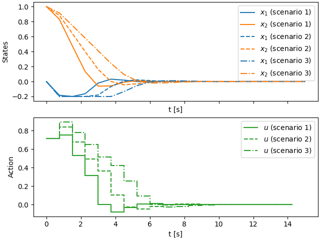
For plotting, we will plot the results in a two axes, one for the states and one for the action. Different scenarios are assigned different linestyles.

fig, axs = plt.subplots(2, 1, constrained_layout=True, sharex=True)

t = np.linspace(0, T, N + 1)
for i, ls in zip(range(K), cycle(["-", "--", "-."])):
    x = sol.value(msmpc.states_i(i)["x"]).toarray()
    u = sol.value(msmpc.actions_i(i)["u"]).toarray().flatten()
    axs[0].plot(t, x[0], ls=ls, color="C0", label=f"$x_1$ (scenario {i + 1})")
    axs[0].plot(t, x[1], ls=ls, color="C1", label=f"$x_2$ (scenario {i + 1})")
    axs[1].step(
        t[:-1], u, ls=ls, color="C2", where="post", label=f"$u$ (scenario {i + 1})"
    )

axs[0].set_ylabel("States")
axs[1].set_ylabel("Action")
for ax in axs:
    ax.set_xlabel("t [s]")
    ax.legend()
plt.show()